Vector Area Zonal Stats Tutorial

A basic introduction to vector area zonal stats

Basic Usage

Generate area zonal stats for a GeoDataframe containing areas of interest with a vector data source containing areas associated with statistics.

Note

The assumption for the data is that the statistics are uniformly distributed over the entire area for each row in the data source.

import geopandas as gpd
import matplotlib.pyplot as plt
import geowrangler.area_zonal_stats as azs

Simple Grid AOIs and Data

simple_aoi = gpd.read_file("../data/simple_planar_aoi.geojson")
simple_data = gpd.read_file("../data/simple_planar_data.geojson")

Given an AOI (simple_aoi) and geodataframe containing sample data (simple_data)

simple_aoi

	geometry
0	POLYGON ((0 0, 0 1, 1 1, 1 0, 0 0))
1	POLYGON ((1 0, 1 1, 2 1, 2 0, 1 0))
2	POLYGON ((2 0, 2 1, 3 1, 3 0, 2 0))

simple_data

	population	internet_speed	geometry
0	100	20.0	POLYGON ((0.25 0, 0.25 1, 1.25 1, 1.25 0, 0.25...
1	200	10.0	POLYGON ((1.25 0, 1.25 1, 2.25 1, 2.25 0, 1.25...
2	300	5.0	POLYGON ((2.25 0, 2.25 1, 3.25 1, 3.25 0, 2.25...

In order correctly apportion the statistic, we need to make sure that the AOI and data geodataframes are using a planar CRS (i.e., gdf.crs.is_geographic == False)

simple_aoi.crs

<Projected CRS: EPSG:3857>
Name: WGS 84 / Pseudo-Mercator
Axis Info [cartesian]:
- X[east]: Easting (metre)
- Y[north]: Northing (metre)
Area of Use:
- name: World between 85.06°S and 85.06°N.
- bounds: (-180.0, -85.06, 180.0, 85.06)
Coordinate Operation:
- name: Popular Visualisation Pseudo-Mercator
- method: Popular Visualisation Pseudo Mercator
Datum: World Geodetic System 1984 ensemble
- Ellipsoid: WGS 84
- Prime Meridian: Greenwich

simple_data.crs

<Projected CRS: EPSG:3857>
Name: WGS 84 / Pseudo-Mercator
Axis Info [cartesian]:
- X[east]: Easting (metre)
- Y[north]: Northing (metre)
Area of Use:
- name: World between 85.06°S and 85.06°N.
- bounds: (-180.0, -85.06, 180.0, 85.06)
Coordinate Operation:
- name: Popular Visualisation Pseudo-Mercator
- method: Popular Visualisation Pseudo Mercator
Datum: World Geodetic System 1984 ensemble
- Ellipsoid: WGS 84
- Prime Meridian: Greenwich

ax = plt.axes()
ax = simple_data.plot(
    ax=ax, color=["orange", "brown", "purple"], edgecolor="yellow", alpha=0.4
)
ax = simple_aoi.plot(ax=ax, facecolor="none", edgecolor=["r", "g", "b"])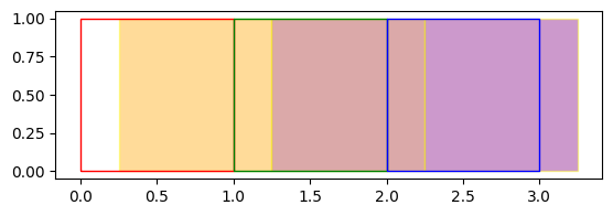

The red, green, and blue outlines are the 3 regions of interest (AOI) while the orange, brown, and purple areas are the data areas.

empty_aoi_results = azs.create_area_zonal_stats(simple_aoi, simple_data)

If no aggregations are specified, the include_intersect=True arg specifies that the sum of the data areas intersecting our AOI is computed in the column intersect_area_sum.

empty_aoi_results

	geometry	intersect_area_sum
0	POLYGON ((0 0, 0 1, 1 1, 1 0, 0 0))	0.75
1	POLYGON ((1 0, 1 1, 2 1, 2 0, 1 0))	1.00
2	POLYGON ((2 0, 2 1, 3 1, 3 0, 2 0))	1.00

Apportioning aggregated statistics

To aggregate statistics over the AOI areas intersecting with the data areas, the default behavior of “apportioning” the statistic over the intersection of the data area overlapping the AOI area depends on the statistic.

• For sum it apportions the total value of the statistic over the proportion of the data area overlapping the AOI area divided by the total area of the data.
• For mean it apportions the total value of the statistic over the proportion of the data area overlapping the AOI area divided by the total area of the aoi.
• For other statistics, there is no apportioning done and uses the raw statistics from the data areas overlapping the AOI area.

Note

This default behavior can be overridden by specifying a prefix (e.g., raw_, data_, and aoi_) to the statistic (i.e., func) – e.g. if you wish the apportion the sum as a proportion of the aoi area instead of the data area, specify the func as aoi_sum instead of sum.

simple_aoi_results = azs.create_area_zonal_stats(
    simple_aoi,
    simple_data,
    [
        dict(func=["sum", "count"], column="population"),
        dict(func=["mean", "max", "min", "std"], column="internet_speed"),
    ],
)

CPU times: user 10.9 ms, sys: 1.13 ms, total: 12 ms
Wall time: 11.3 ms

simple_aoi_results

	geometry	intersect_area_sum	population_sum	population_count	internet_speed_mean	internet_speed_max	internet_speed_min	internet_speed_std
0	POLYGON ((0 0, 0 1, 1 1, 1 0, 0 0))	0.75	75.0	1	15.000	20.0	0.0	NaN
1	POLYGON ((1 0, 1 1, 2 1, 2 0, 1 0))	1.00	175.0	2	6.250	20.0	10.0	7.071068
2	POLYGON ((2 0, 2 1, 3 1, 3 0, 2 0))	1.00	275.0	2	3.125	10.0	5.0	3.535534

simple_aoi_results.population_sum.sum(axis=None)

np.float64(525.0)

Note the value of the mean of the internet speed for the 1st area above.

While there is one data area overlapping with an internet speed of 20.0 the computed aggregate statistic for the mean is 15.0 due to the apportioning which only accounts for 0.75 (the total AOI area is 1.0) – meaning it assigns a value of 0.0 for the 0.25 area with no overlapping data area.

If you wish to override this behavior and impute the value of the statistic as the means of all the overlapping areas (in proportion to the overlap of their area over the total area of the AOI), you can additionally add a prefix of imputed_ as shown in the next example. Note that adding a prefix doesn’t change the default output column name, which is why we explicitly specified an output column name (internet_speed_imputed_mean in order to differentiate it from the original internet_speed_mean column.

Notice as well that adding a raw_ prefix to the min,max,std statistics doesn’t change their values since by default these statistics don’t use any apportioning (so specifying raw_ is redundant in this case).

Lastly, check the effect of setting of the fix_min arg to False (the default value is True) – since it uses the raw column to compute the min, it is not aware that there are areas in the AOI that have no overlapping data areas and uses the min value from the overlapping areas (in this case, since there is only 1 partially overlapping area, it uses that as the min value). The fix_min arg “fixes” this by checking if the data areas completely overlap the AOI area and sets the minimum to 0 if there is a portion of the AOI area that is not completely intersected by a data area.

corrected_aoi_results = azs.create_area_zonal_stats(
    simple_aoi,
    simple_data,
    [
        dict(func=["sum", "count"], column="population"),
        dict(
            func=["mean", "imputed_mean", "raw_max", "raw_min", "raw_std"],
            column="internet_speed",
            output=[
                "internet_speed_mean",
                "internet_speed_imputed_mean",
                "internet_speed_max",
                "internet_speed_min",
                "internet_speed_std",
            ],
        ),
    ],
    fix_min=False,
)

CPU times: user 12.6 ms, sys: 908 µs, total: 13.5 ms
Wall time: 13.5 ms

corrected_aoi_results

	geometry	intersect_area_sum	population_sum	population_count	internet_speed_mean	internet_speed_imputed_mean	internet_speed_max	internet_speed_min	internet_speed_std
0	POLYGON ((0 0, 0 1, 1 1, 1 0, 0 0))	0.75	75.0	1	15.000	20.000	20.0	20.0	NaN
1	POLYGON ((1 0, 1 1, 2 1, 2 0, 1 0))	1.00	175.0	2	6.250	6.250	20.0	10.0	7.071068
2	POLYGON ((2 0, 2 1, 3 1, 3 0, 2 0))	1.00	275.0	2	3.125	3.125	10.0	5.0	3.535534

Custom Grids over admin area data

Another example using aggregated statistics over admin areas (barangay level) that are apportioned into grid areas by their overlap.

Notice that since the grid areas does not completely overlap the admin areas (and vice versa) , the sum of their total populations and land areas are not equal.

region3_admin_grids = gpd.read_file("../data/region3_admin_grids.geojson")
region3_admin_grids = region3_admin_grids.to_crs("EPSG:3857")  # convert to planar

CPU times: user 18.8 ms, sys: 1.53 ms, total: 20.4 ms
Wall time: 20.5 ms

region3_pop_bgy_level = gpd.read_file("../data/region3_population_bgy_level.geojson")

CPU times: user 139 ms, sys: 2.86 ms, total: 142 ms
Wall time: 142 ms

aoi_result = azs.create_area_zonal_stats(
    region3_admin_grids,
    region3_pop_bgy_level,
    [
        dict(func=["sum", "count"], column="population"),
    ],
)

CPU times: user 270 ms, sys: 3.53 ms, total: 274 ms
Wall time: 275 ms

aoi_result

	x	y	geometry	intersect_area_sum	population_sum	population_count
0	0	30	POLYGON ((13334497.956 1771012.807, 13339497.9...	1.213773e+06	687.832840	1
1	0	31	POLYGON ((13334497.956 1776012.807, 13339497.9...	2.471924e+06	986.890853	1
2	0	32	POLYGON ((13334497.956 1781012.807, 13339497.9...	2.748813e+06	1097.435840	1
3	1	30	POLYGON ((13339497.956 1771012.807, 13344497.9...	1.081669e+06	468.368614	2
4	1	32	POLYGON ((13339497.956 1781012.807, 13344497.9...	8.941593e+04	8.570604	2
...	...	...	...	...	...	...
1069	54	44	POLYGON ((13604497.956 1841012.807, 13609497.9...	1.976718e+05	15.398162	1
1070	54	45	POLYGON ((13604497.956 1846012.807, 13609497.9...	1.019141e+07	1613.913393	3
1071	54	46	POLYGON ((13604497.956 1851012.807, 13609497.9...	3.129991e+06	1033.997979	2
1072	54	47	POLYGON ((13604497.956 1856012.807, 13609497.9...	8.106461e+06	250.893691	2
1073	54	48	POLYGON ((13604497.956 1861012.807, 13609497.9...	1.928818e+07	299.377987	3

1074 rows × 6 columns

(
    aoi_result.geometry.area.sum(),
    aoi_result.intersect_area_sum.sum(),
    aoi_result.population_sum.sum(),
)

(np.float64(26850000000.000042),
 np.float64(24548891899.414997),
 np.float64(12136959.090018272))

(region3_pop_bgy_level.geometry.area.sum(), region3_pop_bgy_level.population.sum())

(np.float64(27658006631.682587), np.int64(13139695))

gdf = region3_admin_grids
gdf2 = region3_pop_bgy_level

ax = plt.axes()
ax = gdf2.plot(ax=ax, column="population", alpha=0.4)
ax = gdf.plot(ax=ax, facecolor="none", edgecolor="blue", alpha=0.4)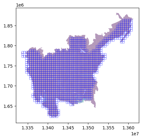

ax = plt.axes()
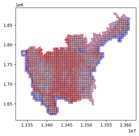
ax = gdf2.plot(ax=ax, facecolor="none", alpha=0.4, edgecolor="red")
ax = aoi_result.plot(column="population_sum", ax=ax, alpha=0.4, edgecolor="blue")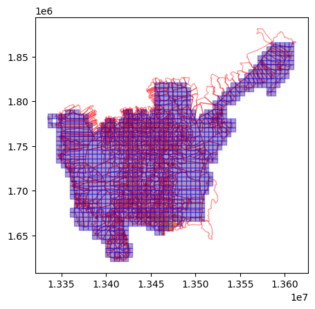

ax = plt.axes()
ax = gdf2.plot(ax=ax, column="population", alpha=0.4, edgecolor="red")
ax = aoi_result.plot(column="intersect_area_sum", ax=ax, alpha=0.4, edgecolor="blue")